
The development of digital technologies has given companies a huge choice of IT tools that help them manage various processes. We are talking about both basic, relatively simple ones such as internal orders, leave requests, as well as highly advanced ones, e.g. manufacturing process management. However, this does not change the fact that Excel is still very often used to run them. Heck – in many cases there is nothing wrong with that! Regarding this, the hero of the next blog post in the „#Top5" series is a popular spreadsheet. It has got many hidden, useful features – and we are not talking here about formulas. Here are five features which will make your daily work much more enjoyable.
Focus cell – how not to get lost in the data
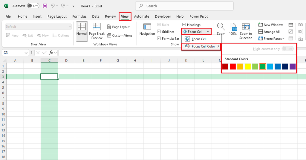
The first feature is called Focus Cell. It works great when you are working with a spreadsheet with a lot of data. Of course – it is easy to get lost in such a spreadsheet. Focus Cell solves this problem. How to use it?
- Open an Excel file.
- Click „View” tab and in „Show” group select „Focus cell”.
This will mark the column and row with the default color and show selected cell. The color is a matter of taste, but if green doesn’t suit you, you can set another one from the available ones:
Navigation – sheets under control
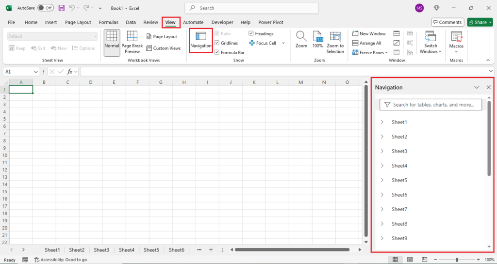
We remain in the section related to the view. Sometimes your spreadsheet has a huge amount of data but there is not only one sheet – there are many of them. It is difficult to find a way around them or switch between them to check the data – the bar at the bottom of the screen turns out to be ineffective. The solution to this problem is the Navigation feature. It is in the same place as the previous one – Focus Cell. So, with the Excel file open:
- Make sure you are in the „View” tab.
- Select „Navigation” in the „Show” group.
As you can see, an additional window – navigation pane – has appeared on the right side of the screen. You can easily use it to switch between sheets quickly and even search for tables and charts that are in them.
New checkboxes
The third feature may not seem groundbreaking. Why? Because at first glance, when we see checkboxes in Excel, we think, "wait a second, that’s nothing new, they’ve been available for a quite long time." That’s true, but some time ago Microsoft decided to introduce completely new checkboxes that have much more to offer. How to use them?
- Create a sample table in Microsoft Excel e.g. to-do list. “Task” and “Status” columns are enough.
- Add checkboxes in “Status” column. To do it, select all cells in mentioned column, click ”Insert” tab in the ribbon and then ”Checkboxes” in ”Controls” group.
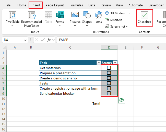
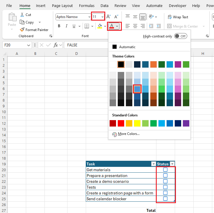
- As you can see, checkboxes have been added. You can easily format them. When cells with checkboxes are selected, go to “Home” tab and change a font color – borders of checkboxes will change. Changing a font size will also change the size of checkboxes.
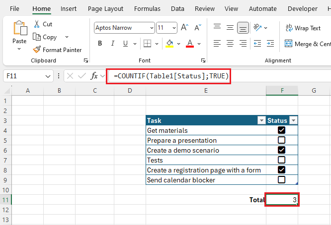
- It is worth mentioning that an empty checkbox has the logical value: ”False” when it is empty and “True” when checked. Thanks to this, they can be used in various calculation formulas. In our example, the ”COUNTIF” formula fits perfectly – it will sum the number of completed tasks from our list (checked checkboxes). The formula with the effect is shown below on the screen.
Picture from file – OCR by Microsoft Excel
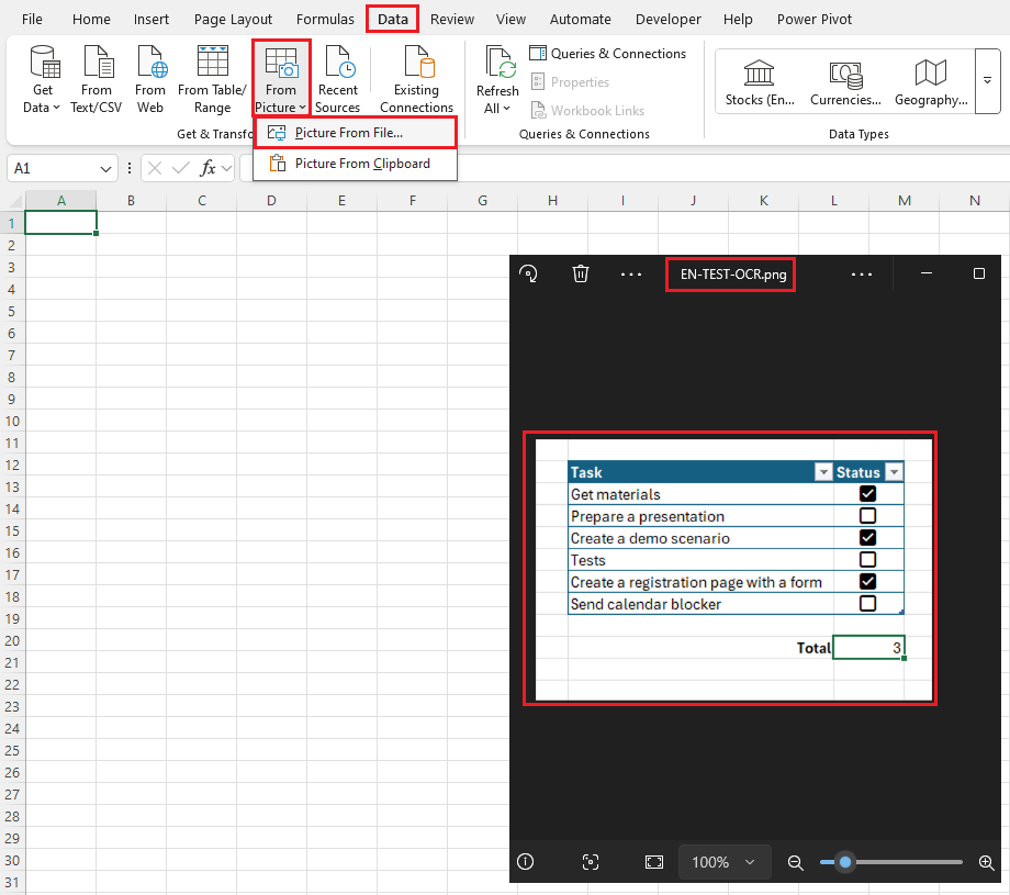
The feature number four may be called a gamechanger. We are talking about the Picture from file option. It is useful, for example, when someone has taken a photo or screenshot of a data table and asks you to enter it into Excel. If there is a lot of data, it would be ideal if Excel recognizes the content from the image and insert it in an editable form into the sheet. Something like OCR, which is often used in ERP systems such as Dynamics 365 Business Central. However - how to use "Excel OCR"?
- While in Excel, select a cell where the data should appear, click the ”Data” tab, then ”From picture”, ”Picture from file…” and choose a picture you want. For demonstration purposes, we have prepared a screenshot of the table from the previously described feature and saved it as .png.
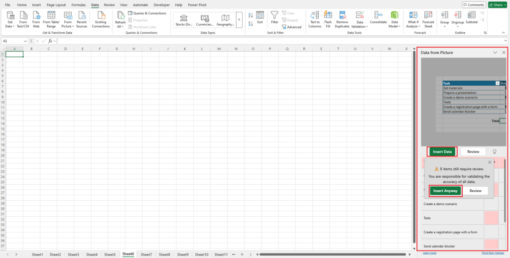
- After selecting the picture, a window with data from the image will be displayed on the right side of the screen. As you can see, we have a preview of the picture and at the bottom, the data that Excel extracted from it. The ones marked red are the ones you should check and accept if Excel recognized them correctly. When you click on any red field it also corresponds to a text on the image. You do not have to confirm all the fields individually – just click the "Insert data" and "Insert anyway" buttons.
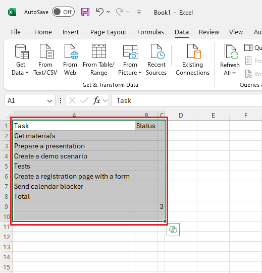
- As you can see, the data from the picture has been added to the spreadsheet – it just needs to be formatted appropriately. Do you think Excel could handle a photo with handwriting? Check it out and share your results!
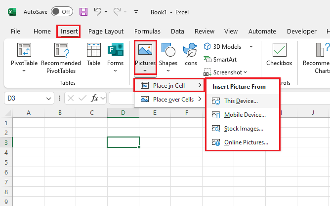
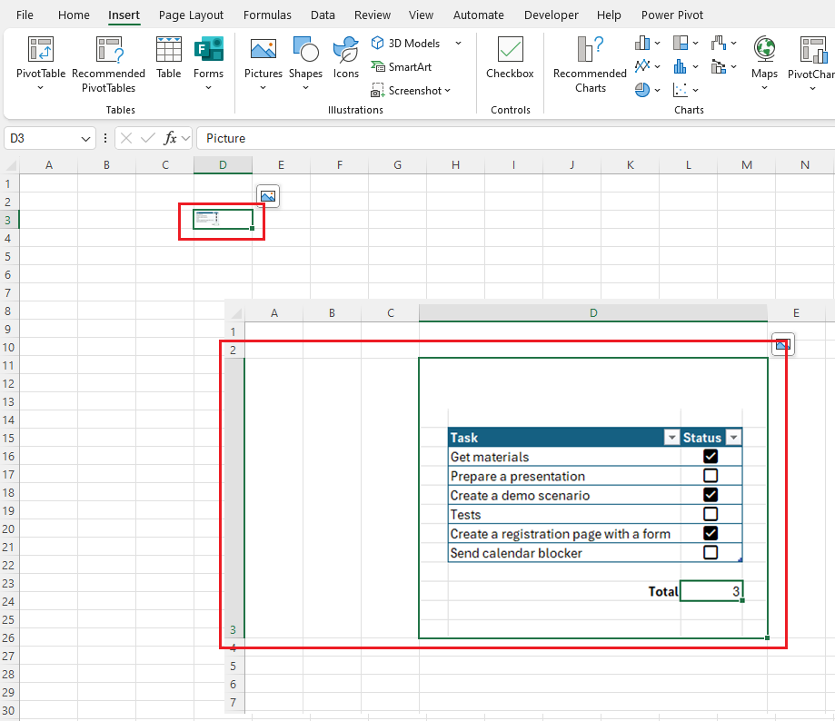
Insert picture in cell
Sometimes we need to add a picture to a spreadsheet. And almost always there is a problem with adjusting the size of individual image to a cell. In such cases, it is worth using the Place in cell feature. Using it will cause the photo to automatically adjust its size to a cell. The best way to get to know this feature is with an example.
- Open an Excel spreadsheet and select an empty cell.
- Next, go to ”Insert” tab, select ”Pictures”, ”Place in Cell” and select a picture you want to add.
- As you can see, it has been reduced to the size of a cell but modifying its size also affects the size of the added photo.
If you would like to talk about the presented features, you have the impression that they do not work properly in your Microsoft Excel or you are curious about what else is hidden in the spreadsheet – do not wait, contact us and arrange a free consultation with our specialist, who will provide you with the necessary information. Oh – and do not forget to follow the next blog posts from our “#Top5” series.
